Iot (Internet of Things) and ArcGIS GeoEvent

IoT is the buzz word these days. Everyone wants to tap into the IoT data streams and build analytic apps. The growth of IoT devices over the next few years is shown below.growth-iot

IoT apps range from, a baby monitor, telling which lighting conditions or lullaby your baby likes best when sleeping to a predictive maintenance app that monitors array of electric instrumentation for energy demand forecasting and tier pricing.

A device or thing in the IoT world is a piece of hardware such as light or motion sensor that measures a phenomenon  such as light intensity, temperature and humidity. These devices need to be connected to the Internet to harness the real power. Commons protocols for data transport are HTTP, MQTT and AMQPS.

Major IoT providers are Microsoft IoT suite, IBM Watson IoT and Amazon IoT. These providers have hub and sdks. Hubs provide infrastructure for brokers to store and forward messages from publishers to subscribers and vice-versa in a secure and scalable fashion. Not all IoT providers support storage (message retention). The incoming messages can be saved to external storage such as HDFS, S3, or Dynamo

SDKs provide APIs for publishing and consuming. Some of the popular ones are Raspberry PI and Arduino device SDKs, here.

Topic/queues are used to publish and receive messages. A topic such as “/grid1/device/reading/area1” can be used to receive readings from electric meters in area1. The messages can be analyzed in real-time or batch mode, the heart of analytics.

Rules can be created using Lambda functions to filter incoming messages and stored in Amazon Dynamo or re-publish to a different topic.

The communication between the devices and the apps can be duplex. This functionality is supported though Shadow API, that lets apps control the devices to take certain actions such as turn a valve off if the temperature exceeds a threshold value.

Special topic like this $aws/things/myElectricMeter/shadow/update are reserved for shadow updates.

A topic can be used as a gateway for hundreds of devices. Each device needs to have its own certificate that can be generated using AWS CLI or AWS SDK.

Esri’s  GeoEvent is  a product that provides real-time capability to monitor assets such as fleet vehicles and response to events.

Geoevent framework can be leveraged to plugin new data streams though providing a transport and adapter.

Transport encapsulate the semantics of inbound/outbound communication (mqtt, http, amqs.etc) with external hubs such as AWS and Azure IoT hubs. Adapter encapsulates the message format that need to be read and processed in geojson, avro etc. Some of the existing transports, processors and adapters can be found here

AWS transport for geoevent can be found here.

Cmd tools to publish and consume messages from AWS IoT hub are available here(Java and Scala). A GUI app is available here,

In the next post post I will show how to use GE Processsor to leverage Spark streaming and perform machine learning and analytics.

Near realtime tweet language and sentiment detect using Kafka, Spark Streaming and Elastic Search

In the post we will use Spark streaming to fetch tweets from a kafka topic, calculate the tweet sentiment and language and create search index and perform some aggregations.

We will fetch tweets using Twitter API and use  Kafka Producer to feed a topic, use Spark streaming to get the tweets from Kafka topic and calculate sentiment and language detect using Stanford CoreNLP.  Avro is used to serialize tweets.
Tweet schema:
{
"namespace": "com.esri.avro",
"type": "record",
"name": "Tweet",
"fields": [{
"name": "name",
"type": "string"
}, {
"name": "text",
"type": "string",
"avro.java.string": "String"
}, {
"name": "language",
"type": "string",
"avro.java.string": "String"
}, {
"name": "score",
"type": "int",
"default": 0
}]
}

Register the avro Tweet with Spark’s KryoSerialier

sparkConf.set("spark.serializer", "org.apache.spark.serializer.KryoSerializer")
sparkConf.registerKryoClasses(Array(classOf[Tweet]))

Followed by populating a search index in ElasticSearch and perform aggregations and visualizations using Marvel and Kibana Also fine tune Elastic Search’s text analyzers to retrieve better results.

Summary workflow:
kafka_spark_es_flow

Steps:

1. Script to fetch tweets
Python script uses tweepy streaming API to fetch tweets, extracts the text and pipes to Kafka console producer

2. Kafka console producer
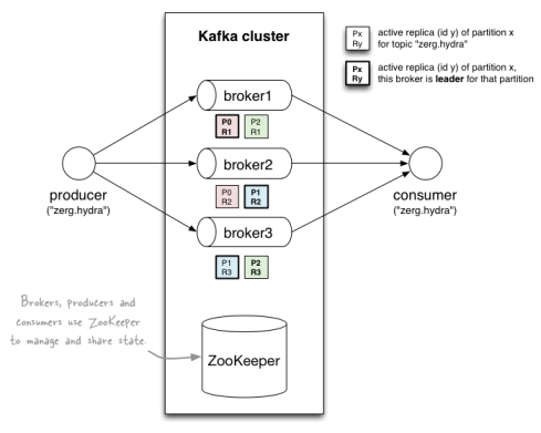
The producer populates a kafka topic with live tweets.
kafka-arch

3. Spark streaming, CoreNLP
Spark streaming is used to retrieve live tweets from a Kafka topic, detect language and sentiment using CoreNLP and store to search Index

4. Elastic Search
Marvel and Kibana are used to perform aggregations and visualizations.
POST user_tweets
{
"settings": {
"index": {
"number_of_shards": 5
}
},
"mappings": {
"sentiments": {
"properties": {
"language": {
"type": "string"
},
"score": {
"type": "integer"
},
"text": {
"type": "string"
},
"name": {
"type": "string"
}
}
}
}
}POST user_tweets
{
"settings": {
"index": {
"number_of_shards": 5
}
},
"mappings": {
"sentiments": {
"properties": {
"language": {
"type": "string"
},
"score": {
"type": "integer"
},
"text": {
"type": "string"
},
"name": {
"type": "string"
}
}
}
}
}

Marvel cluster stats:
es_marvel_cluster

Sentiment score distribution
es_marvel_hist_sentiment

Tweet Language count:es_marvel_language_group

Kibana: Histogram of Tweets every 30 secs

movie_tweets_hist

Line chart of tweets indexed every second

movie_tweets_sec_linechart

Histogram of tweets with high sentiment score

movie_tweets_top_senti

Pie Chart (donut) number of tweets by language

movie_tweets_top10lang

Code can be found on Git

Top k users using algebird bloomfilter in Spark

This analysis involves picking the top k users with high spending potential for marketing purposes.
Dataset description:

  • Users: list of user information, userid, name, email, phone numbers
  • Transactions: transactions for each user, userid, dollar spent, datetime
  • Do-Not-call: List of user phones numbers who do not wish to be called.

Task: To find top K users with spending potential both the users and transactions data need to be joined. Join is an expensive operation. Here are a couple of approaches:

    a. Filter the users based on do-no-call list. Only allow users who like to hear about marketing/promotions. If the resulting users list is small enough to fit in memory, we can cache/replicate (broadcast in Spark) on all the nodes in the cluster for use during join with transactions.
    b. If the user list will not fit in-memory, we can create a bloom filter to reduce the size of the users, broadcast the BF to nodes and filter the transactions. This will reduce number of transactions during the final join operation.

Bloom Filter is size efficient, probabilistic data structure that is used to validate set membership. They eliminates false negatives but might have false positives due to hash collisions.

Bloom filter are also Monoids. A monoid is an algebraic data structure with following 3 properties where there is,
1. A binary operation take two values of type T and return a value of type T.
2. An identify element must exist that when used against the binary operation must yield same type T. (zero for addition, 1 for multiplication)
3. Associative.Changing the order of operands should not change the end result. e.g operations such as addition or multiplication. (subtraction, mean are not associative). This is useful when performing operations on large datasets in a distributed fashion as it helps of operations such as combine at mapper level and decreases the intermediate data (network traffic) that needs to be shuffled to reducers.
class Monoid {
def Op(x:T, y:T): T
def identity : T
}

At a high level, a bloom filter is a bit vector that computes k hashes values (Jenkins or Murmur hash) for an item and stores the k hash values at computed index locations in the bit vector. Check for set membership of an item is a read/AND operation of all the hash collisions obtained by computing k hashes for the item.

Process:

  • Step 1: Read input datasets and clean up.
    Filter users who do not have valid phone numbers and email addresses. Filter transactions to remove $ sign from amount spent.
  • Step 2: Filter the users based on do-not-call list
  • Step 3: Create BloomFilterMonoid for users based on userid.
    Broadcast the users BF to all the nodes in the cluster.
  • Step 4: Aggregate transactions by user.
    Marketing is based on 2015 year. So filter transactions for year 2015, use reduce operation to aggregate the total dollar amount spent by each users.
  • Step 5: Filter the transactions using user BloomFilter (from step3).
    Users BF is used to filter transactions to reduce number of transactions for later join.
  • Step 6: Finally join users and (filtered) transactions and project
  • Step 7: Sort by dollar amount spent in descending order and take k users.

The code can be found on Git.

Loan Data Prediction using Spark Mllib Logistic Regression

In this post I will analyze loan prediction model using Logistic Regression algorithm and evaluate it using LogLoss function.

  • Step 1: Prosper loan data description

The loan data can be found here. We will use following predictors to build our model.
Target variable:
LoanStatus
Predictors:
EmploymentStatus - The employment status of the borrower at the time they posted the listing.
EmploymentStatusDuration - The length in months of the employment status at the time the listing was created.
IsBorrowerHomeowner - Is the borrower own a home
LoanOriginalAmount - The origination amount of the loan.
AmountDelinquent - Dollars delinquent at the time the credit profile was pulled.
DelinquenciesLast7Years - Number of delinquencies in the past 7 years at the time the credit profile was pulled.
CreditScoreRangeLower - The lower value representing the range of the borrower's credit score as provided by a consumer credit rating agency.
StatedMonthlyIncome - The monthly income the borrower stated at the time the listing was created.
DebtToIncomeRatio - The debt to income ratio of the borrower at the time the credit profile was pulled.

  • Step 2: Parse and featurize

This step will parse the data and created data point. Each data point is of type LabeledPoint
The target variable LoanStatus is considered good (represented as 1.0) for following: Current, Completed, FinalPaymentInProgress, Cancelled.
We have used one categorical predictor for use in the model, IsBorrowerHomeowner. The Boolean True or False are replaced with dummy variables 1.0 and 0.0 respectively. If there are large number of categorical variables in modeling, encoding techniques such ONE-HOT-Encoding can be used like in my other post here.

  • Step 3: Split data into training, validation and test sets.

val splits = labeledPointsGood.randomSplit(Array(0.8, 0.1,0.1))

Training data is used to train base modelValidation data is used to evaluate model performance and choose best model with minimum logloss using grid searchTesting data is used for prediction using the best model

  • Step 4: Train the LogisticRegression Model. Perform grid search to find best hyper-parameters and model using validation dataset using logloss function.
    • Step 5: Evaluate test data set logloss using the best model.

Calculate ROC (Area Under the Curve) and model weights to find out which predictors influences the target variable the most. The Area under curve: 0.923884. ROC curve show trade-off between false-positive rate and true-positive rate. I used scala-chart to plot the ROC curve.

ROC Curve

ROC Curve

    The model weights with higher value contribute towards the target variable. EmploymentStatus and IncomeToAmountRatio are two predictors with higher weights.

Model Weights:
-0.10488689221891605
1.2278111772823685
6.8045639548692E-4
1.56480139828527E-5
-4.998426314141764E-6
-0.01029075526067838
0.001283343807366695
2.662548287482352E-5
0.042455998070836644
-0.15168601961643607

The code can be found on Git

NYC taxi trip density map using Spark

This analysis will use the NYC taxi cab trips data to compute density rasters.
The data can be obtained here.
Each record is in the following structure,
medallion,hack_license,vendor_id,rate_code,store_and_fwd_flag,pickup_datetime,
pickup_latitude,dropoff_longitude,dropoff_latitude

Data columns for interest are taxi id(medallion), pickup/dropoff datetime, pickup/dropoff longitude/latitude, trip_time and trip_distance.
Sample trip:
AECF13C3F540D4CF4,BA96DE419E711691B9445D6A6307C170,CMT,1,N,2013-01-01 15:11:48,2013-01-01 15:18:10,4,382,1.00,-73.978165,40.757977,-73.989838,40.751171
1. Data representation
The raster data format is used to represent continuous phenomenon such as temperature and precipitation.
More information about raster data format can be found here. To generate a density raster following information is needed,

  • a. bounding box of the area/raster (xmin, ymin, xmax, ymax)
  • b. cell width, height
  • c. spatial reference
    Using this information number of rows and columns of the raster can be determined using following formula,
    rows = ymax - ymin/cell_size
    cols = xmax - xmin/cell_size

2. Data parsing

  • a. Parse the taxi record and calculate row, column for the taxi pickup longitude/latitude using following formula,
    col = trip_pickup_longitude - xmin /cell_size
    row = trip_pickup_latitude - ymax / cell_size
  • b. Parse the taxi trip pickup datetime to generate yyyyMMddHH, so that we can aggregate by hour later
  • c. Generate following tuple for each taxi record,
    ((row, col, yyyyMMddHH),1)

Here is the parse code, similar to my other post that calculates average daily speed of a taxi.
raw_data_input = sc.textFile("/spark/nyc-taxi/data/trip_data_test_1.csv")
trips = raw_data_input.map(ingest_record)
def ingest_record(record):
"""
Args:
record (str) - taxi record
Returns
((int, int, str), int) - ((row, col, yyyyMMddHH), 1)
"""
(medallion, hack_license, vendor_id, rate_code, store_and_fwd_flag,
pickup_datetime, dropoff_datetime, passenger_count, trip_time_in_secs,
trip_distance, pickup_longitude, pickup_latitude, dropoff_longitude,
dropoff_latitude) = record.split(',')
pickup_date, pickup_time = pickup_datetime.strip().split()
pickup_year, pickup_month, pickup_day = pickup_date.split(‘-‘)
pickup_hour, pickup_minute, _ = pickup_time.split(‘:’)
row, col = get_row_col(pickup_datetime)
yyyyMMddHH= “{pickup_year}{pickup_month:02d}{pickup_day:02d}{pickup_hour:02d}”.format(
pickup_year=int(pickup_year), pickup_month=int(pickup_month), pickup_day=int(pickup_day),
pickup_hour=int(pickup_hour))
return ((row, col, yyyyMMddHH), 1)

3. Aggregate
In this step well we will create an hourly aggregation of taxi trips using reduceByKey
trips.reduceByKey(sum)
The result of hourly aggregation is RDD with following elements:
[((162, 616, '2013011309'), 2), ((771, 209, '2013011316'), 1), ((361, 911, '2013011317'), 1), ((343, 921, '2013011317'), 1), ((253, 830, '2013011313'), 2), ((60, 662, '2013011305'), 1), ((78, 463, '2013011311'), 1), ((82, 590, '2013011312'), 1), ((87, 587, '2013011312'), 1), ((90, 555, '2013011311'), 1)]

4. Create raster from trips
Results from aggregation is of following format: ((row, col, yyyyMMddHH), aggr_val)
To create a raster,

  • Generate tuple to aggregate by yyyyMMddHH -> (yyyyMMddHH, (row, col, aggr_val))
  • Create a numpy 2d array (dimension nrows x ncols – 800X800 in our example) where each element represents aggregation value.

Output of this step,
[('2013010102', array([[ 0., 0., 0., ..., 0., 0., 0.],
[ 0., 0., 0., ..., 0., 0., 0.],
[ 0., 0., 0., ..., 0., 0., 0.],
...,
[ 0., 0., 0., ..., 0., 0., 0.],
[ 0., 0., 0., ..., 0., 0., 0.],
[ 0., 0., 0., ..., 0., 0., 0.]], dtype=float32)),
('2013010103', array([[ 0., 0., 0., ..., 0., 0., 0.],
[ 0., 0., 0., ..., 0., 0., 0.],
[ 0., 0., 0., ..., 0., 0., 0.],
...,
[ 0., 0., 0., ..., 0., 0., 0.],
[ 0., 0., 0., ..., 0., 0., 0.],
[ 0., 0., 0., ..., 0., 0., 0.]], dtype=float32)),

5. Plot the density map
Use the matplot to plot the density.
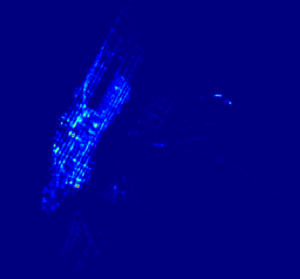
1-hr density
1hr-density
4hr density
geohash-density-8

Click through rate (CTR) prediction using Spark

Predicting whether a person is going to click on a advertized link is a billion dollars industry. In this analysis we will predict whether a user clicks on link using Naive Bayes algorithm. I have chosen to use Kaggle Avazu CTR data here.
We will go through the process of parsing, featurizing (using OHE – One-Hot-Encoding),
modeling, evaluating and prediction steps.
Steps:
1. Parsing
Data format has following attributes:
id,click,hour,C1,banner_pos,site_id,site_domain,site_category,app_id,app_domain,
app_category,device_id,device_ip,device_model,device_type,device_conn_type,
C14,C,C16,C17,C18,C19,C20,C21
1000009418151094273,0,14102100,1005,0,1fbe01fe,f3845767,28905ebd,ecad2386,
7801e8d9,07d7df22,a99f214a,ddd2926e,44956a24,1,2,15706,320,50,1722,0,35,-1,79
id - ad identifier
click - 1-click/0-non-click
hour - YYMMDDHH

Split the data into train and test sets using randomSplit() function
var ctrRDD = sc.textFile("../click-predict/data/ctr-avazu.csv");
var train_test_rdd = ctrRDD.randomSplit(Array(0.8, 0.2), seed = 37L)
var train_raw_rdd = train_test_rdd(0)
var test_raw_rdd = train_test_rdd(1)
println("Train records : " + train_raw_rdd.count)
println("Test records : " + test_raw_rdd.count)
train_raw_rdd.cache()
test_raw_rdd.cache()
Total records : 131068
Train records : 104920
Test records : 26148

2. Featurize One-Hot-Encoding
We will parse each line, tokenize each data point. Each data point will be a list of tuples like
(featureId, feature).
Ignore the Ad id and target variable, the following tuples are created for the data point below.
1000009418151094273,0,14102100,1005,0,1fbe01fe,f3845767,28905ebd,ecad2386,
7801e8d9,07d7df22,a99f214a,ddd2926e,44956a24,1,2,15706,320,50,1722,0,35,-1,79
Data point tuples
(0,14102100)
(1, 1005)
(2, 0)
(3, 1fbe01fe)
(4,f3845767)
...

OHE process creates a dictionary of unique features – tuples in our case like -> (featureId, feature). Categorical features range from 5-13.
var train_rdd = train_raw_rdd.map{ line => var tokens = line.split(",")
var catkey = tokens(0) + "::" + tokens(1)
var catfeatures = tokens.slice(5, 14)
var numericalfeatures = tokens.slice(15, tokens.size-1)
(catkey, catfeatures, numericalfeatures)
}
// create one-hot-encoding dictionary
var oheMap = train_rdd.map(x => x._2).flatMap(x => x).distinct().zipWithIndex().collectAsMap()

distinct, removes duplicate elements in an RDD
zipWithIndex, zips elements in the feature rdd with unique index. The resulting dictionary will look as below:
{(10, u'8daee47e'): 0, (9, u'28dd2eaa'): 1, (9, u'ce836eb4'): 2, (3, u'8c788ce9'): 3, (9, u'9b90a4bb'): 4, (10, u'd7ecb33e'): 5, (3, u'2b1ddb24'): 6, (10, u'83f656a4'): 7, (10, u'd8225440'): 8, (10, u'15b894e0'): 9, (10, u'420e4522'): 10, (10, u'06656ab5'): 11,.....

OHE dictionary keys : 58383 (number of unique categorical features in the training set)
Use the OHE dictionary to encode training data to generate a dense vector representation of features. A Sparse vector represents is more appropriate when dealing with large feature vectors since only vector size,
indexes, data values (that belong to indexes) are stored.
var ohe_train_rdd = train_rdd.map{ case (key, cateorical_features, numerical_features) =>
//parse catagorical features
var cat_features_indexed = parseCatFeatures(cateorical_features)
var cat_feature_ohe = new ArrayBuffer[Double]
for (k <- cat_features_indexed) {
if(oheMap contains k){
cat_feature_ohe += (oheMap get (k)).get.toDouble
}else {
cat_feature_ohe += 0.0
}
}
var numerical_features_dbl = numerical_features.map{x => var x1 = if (x.toInt < 0) "0" else x
x1.toDouble}
var features = cat_feature_ohe.toArray ++ numerical_features_dbl
LabeledPoint(key.split("::")(1).toInt, Vectors.dense(features))
}
//parse categorical variables
def parseCatFeatures(catfeatures: Array[String]) : List[(Int, String)] = {
var catfeatureList = new ListBuffer[(Int, String)]()
for (i catfeatures(i).toString
}
catfeatureList.toList
}

Next, create LabeledPoint as input for machine learning models.
LabeledPoint for a single data point can be presented as follows:
[LabeledPoint(0.0,[43104.0,21179.0,28623.0,42373.0,31163.0,14856.0,52422.0,54125.0,
46383.0,2.0,15706.0,320.0,50.0,1722.0,0.0,35.0,0.0])

LabeledPoint(1.0, DenseVector)
The predictor ‘C20’ can have negative values some times, since Naive Bayes model needs all the input model parameters to be positive we set the negative to 0.0.

3. Train Naive Bayes Model
var naiveBayesModel = NaiveBayes.train(ohe_train_rdd)

4. Prediction of CTR
base case: model always predicts 1
var predictions_base = ohe_test_rdd.map(lp => 1.0)
predictions_base.take(10).foreach(println)
var predictionAndLabelBase = predictions_base.zip( ohe_test_rdd.map(_.label))
var accuracy_base = 1.0 * predictionAndLabelBase.filter(x => x._1 == x._2 ).count/ohe_test_rdd.count
println("Base Model accuracy " + accuracy_base)
//0.1735=> 17.35%

using Naive Bayes model predictions:
var predictions = ohe_test_rdd.map(lp => naiveBayesModel.predict(lp.features))
predictions.take(10).foreach(println)
var predictionAndLabel = predictions.zip( ohe_test_rdd.map(_.label))
var accuracy = 1.0 * predictionAndLabel.filter(x => x._1 == x._2 ).count/ohe_test_rdd.count
println("Model accuracy " + accuracy)
//0.5740018357044516 => 57.4%

In the next blog post I will use using the same dataset to train Logistic Regression model and evaluate model performance using LogLoss.

Simple document classification using cosine similarity on Spark

The flux of unstructured/text information sources is growing at a rapid pace. Applications such as document classification, fraud, de-duplication and spam detection use text data for analysis. Unstructured data needs to be numericised before it can be input to a machine learning algorithms.
I have chosen to use newsgroups documents at UCI machine learning repository here. This data has 20 newsgroups and each group has documents/messages about topics such as atheism, science, sports and motorcycles.

This analysis will perform document classification to identify if two documents are similar to each other. The metric used to evaluate is cosine similarity.cosine-fn
Steps:
1. Read the newsgroups dataset, cache and count.
text_rdd = sc.wholeTextFiles(root_dir + 'data/mini_newsgroups/*')
text_rdd.cache()
print text_rdd.count()

Output:19997
2. Tokenize and filter for stopwords. Stopwords can be obtained here.
text_tokenized_rdd = text_rdd.map(lambda a : (a[0].split("/")[-2], tokenize(a[1])))
stopwords_rdd= sc.wholeTextFiles(root_dir + 'data/stopwords/*')
stopwords_list_rdd = stopwords_rdd.flatMap(lambda a: tokenize(a[1]))
stopwords_list = (stopwords_list_rdd.distinct().collect())
tokens_rdd = text_tokenized_rdd.map(lambda a: (a[0], remove_stopwords(a[1], stopwords_list)))

output:
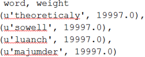
text-tokens

3. Compute the IDF weight of each word in newsgroups corpus. Weights are also known as IDFs (inverse document frequencies). IDFs assigns higher weight to words that are rare across the corpus and vice-versa. So, if two documents share rare words they are considered more likely to have similar content. IDF of a term/word is computed by dividing number of documents in the corpus with number of documents that share the word.
IDF dictionary output:
idfs

4. Document similarity. Calculate Cos similarity between 2 documents from:
Case A. same newsgroup (alt.atheism)
Case B. different newsgroups(alt.atheism, sci.space)
Cosine similarity of two documents can be performed by calculating the dot product of 2 document vectors divided by the product of magnitude of both document vectors.

A document is represented as vector of [(word1, TF-IDF), (word2, TF-IDF),..]
TF-IDF is a measure of importance of a word in a document that is in a corpus.
TF- term frequency (local weight), number of times a term occurs in a document divided by total number of words in the doc
IDF – inverse document frequency( global weight), number of documents in the corpus divided by number of docs with the term

Case A: Use documents from same newsgroup to test similarity
#tokenize and remove stopwords
testdocs1= ['53599','53351'] # alt.atheism
test_sim_tokenize_rdd = text_rdd.filter(lambda a: a[0].split("/")[-1] in testdocs1).map(lambda a : (a[0].split("/")[-1], tokenize(a[1])))
test_sim_cleaned_rdd = test_sim_tokenize_rdd.map(lambda a: (a[0], remove_stopwords(a[1], stopwords_list)))
#calculate tf-idf for both documents.
test_sim_tfidf_rdd = test_sim_cleaned_rdd.map(lambda a: (a[0], tfidf(a[1],idf_weights))).values()
docs = test_sim_tfidf_rdd.collect()
print cosine_similarity(docs[0], docs[1])

The cosine similarity function takes 2 docs and returns similarity measure. Each doc is represented as dictionary, key=word, val=tf*idf
Output Cosine similarity : 0.00107800016479

Case B: Use documents from different newsgroup to test similarity
#repeat steps from case A with documents from different newsgroups
testdocs2= ['53599','59904'] # alt.atheism, sci.space
test_sim_tokenize_rdd = text_rdd.filter(lambda a: a[0].split("/")[-1] in testdocs2).map(lambda a : (a[0].split("/")[-1], tokenize(a[1])))
test_sim_cleaned_rdd = test_sim_tokenize_rdd.map(lambda a: (a[0], remove_stopwords(a[1], stopwords_list)))
#calculate tf-idf for both documents.
test_sim_tfidf_rdd = test_sim_cleaned_rdd.map(lambda a: (a[0], tfidf(a[1],idf_weights))).values()
docs = test_sim_tfidf_rdd.collect()
print cosine_similarity(docs[0], docs[1])
Output Cosine similarity : 0.000529757002339
The Cosine similarity of documents from same newsgroup is higher.

A dictionary represents (term, tf*idf) vector, this approach is not efficient when feature dimensions are large.This problem can be solved by Hashing and SparseVectors. More information can be found here.

Support Vector Machine – SVM for analysis of car acceptability

Scikit-learn is great open-source python library for Machine Learning analysis.
I will use SVM – Support Vector Machine to find car acceptability using car evaluation dataset at UCI ML repository, here.
The dataset has following attributes:
Target:unacc, acc, good, vgood
Predictors:
buying: vhigh, high, med, low.
maint: vhigh, high, med, low.
doors: 2, 3, 4, 5more.
persons: 2, 4, more.
lug_boot: small, med, big.
safety: low, med, high.
We will use the predictors to predict the target variable, the car condition. This is a classification problem.
1. Data exploration
Lets us look at the data first using pandas.
cars = pd.read_csv("data/cars-cleaned.txt", delimiter=",");
cars_head
Target variable: accept – car acceptability
2. Create dummy variables
The predictor variables need to be converted to numeric values before they can be input into ML algorithm.
Following is the encoding scheme:
buying: buying price – vhigh -> 4, high -> 3, med -> 2, low -> 1
maint: maintenance – vhigh -> 4, high -> 3, med -> 2, low -> 1
doors: number of doors – 2 -> 2, 3 -> 3, 4 -> 4, 5more -> 5
persons: persons capacity – 2 -> 2, 4 -> 4, more -> 5
lug_boot: trunk size – small -> 1, med -> 2, big -> 3
safety: safety rating – small -> 1, med -> 2, big -> 3
Transformed dataset:
cars_cleaned
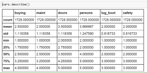
Get basic statistics
cars_describe
3. Create training and test data
cars_y = cars['accept']
cars_x = cars.ix[:,:-1]
train_y, test_y, train_x, test_x = train_test_split(cars_y, cars_x, test_size = 0.3, random_state=33)

4. Train SVM model with linear kernel
model = svm.SVC(kernel="linear", C=0.01)
model = model.fit(train_x, train_y)

5. Predict and plot
y_predictions = model.predict(test_x)
print "Model Accuracy : " , model.score(test_x, test_y)
c_matrix = confusion_matrix(test_y,y_predictions)
print "confusion matrix:"
print c_matrix
plt.matshow(c_matrix)</code>

Model Accuracy: 0.801541425819 (80.1%)
confusion matrix:
[[ 67 0 37 0]
[ 21 0 5 0]
[ 19 0 349 0]
[ 21 0 0 0]]
cars_confusion_matrix

Analysis of NYC Taxi cab data using Spark

Recently I came across of NYC taxi cab drivers data. The data can be obtained here.
Each record is in the following structure,
medallion,hack_license,vendor_id,rate_code,store_and_fwd_flag,pickup_datetime,

pickup_latitude,dropoff_longitude,dropoff_latitude
Data columns for interest are taxi id(medallion), pickup/dropoff datetime, pickup/dropoff longitude/latitude, trip_time and trip_distance.
Sample trip:
AECF13C3F540D4CF4,BA96DE419E711691B9445D6A6307C170,CMT,1,N,2013-01-01 15:11:48,2013-01-01 15:18:10,4,382,1.00,-73.978165,40.757977,-73.989838,40.751171
Question: What is the daily average speed of a taxi ?
Step 1. Parse the data.
Extract medallion, pickup-datetime, trip speed(from trip_time_in_secs, trip_distance)
For each record emit following tuple, (medallion, (yyyyMMddhh,speed))

raw_data_input = sc.textFile("/spark/nyc-taxi/data/trip_data_test_1.csv")
trips = raw_data_input.map(ingest_record)
def ingest_record(record):
"""
Args:
record (str) - taxi record
Returns
(str, (str, float) - taxi id, (yyyyMMddHH, speed)
"""
(medallion, hack_license, vendor_id, rate_code, store_and_fwd_flag,
pickup_datetime, dropoff_datetime, passenger_count, trip_time_in_secs,
trip_distance, pickup_longitude, pickup_latitude, dropoff_longitude,
dropoff_latitude) = record.split(',')

pickup_date, pickup_time = pickup_datetime.strip().split()
pickup_year, pickup_month, pickup_day = pickup_date.split(‘-‘)
pickup_hour, pickup_minute, _ = pickup_time.split(‘:’)
trip_time_in_secs_val, trip_distance_val = int(trip_time_in_secs), float(trip_distance)
if trip_distance_val == 0 or trip_time_in_secs_val == 0:
speed = 0.0
else:
speed = (trip_distance_val * 60 * 60)/trip_time_in_secs_val
yyyyMMddHH= “{pickup_year}{pickup_month:02d}{pickup_day:02d}{pickup_hour:02d}”.format(
pickup_year=int(pickup_year), pickup_month=int(pickup_month), pickup_day=int(pickup_day),
pickup_hour=int(pickup_hour))
return (medallion, (yyyyMMddHH, speed))
RDD output:
(‘389499E7F3F1282517DE8BE747388641’, (‘2013011011′, 23.45))
(’20D9ECB2CA0767CF7A01564DF2844A3E’, (‘2013010711’, 5.28))
Step 2. Cache the RDD for further analysis
trips.cache()
Step 3. Filter by a taxi id, XXXE7FFDFXXXXXXXXXXXX
a_taxi_trips = trips.filter(lambda x : x[0] == ‘XXXE7FFDFXXXXXXXXXXXX’)
RDD output:
(‘389499E7F3F1282517DE8BE747388641’, (‘2013010304’, 23.45))
(‘389499E7F3F1282517DE8BE747388641’, (‘2013010312’, 5.21))
(‘389499E7F3F1282517DE8BE747388641’, (‘2013011016’, 3.78))
Step 4: Extract hour and speed. Group and Sort by key. The key is hour
a_trip_days = a_taxi_trips.map(lambda x : (x[1][0][8:], x[1][1])).groupByKey().sortByKey()
print a_trip_days.collect()

RDD output:
[(’03’, ‘15.36’), (’04’, ‘27.84’), (’07’, ‘25.88’), (’08’, ‘29.04’), (’09’, ‘21.45’), (’10’, ‘20.00’), (’11’, ‘19.42’), (’12’, ‘12.21’), (’13’, ‘13.25’), (’14’, ‘12.88’), (’15’, ‘21.38’)]
Step 5. Plot
def plot_taxi_avg_dailyspeed(hours, avg_speeds):
fig = plt.figure(figsize=(8,4.5), facecolor='white', edgecolor='white')
plt.axis([min(hours), max(hours), 0, max(avg_speeds)+10])
plt.xticks(np.arange(min(hours), max(hours)+1, 1.0))
plt.yticks(np.arange(round(min(avg_speeds),0), max(avg_speeds)+10, 5.0))
plt.grid(b=True, which='major', axis='y')
plt.xlabel('Hour')
plt.ylabel('Speed')
plt.title('Average daily taxi speed')
plt.plot(hours, avg_speeds, '--' , color='b', markersize=25)
plt.show()

avg_daily_speed3
The plot show average taxi speed by the hour. Some observations below may be made such as, increase in speed during the early and late hours, decrease in speed approaching zero during shift at 4pm.
This article scratches the surface of data analysis that is possible with Spark.

Spam classification with naive bayes using Spark MLlib

Spark is super fast (10-100x that map reduce) data computing engine that uses memory storage and computation.
MLlib is built on spark, allows to run machine learning algorithms such as clustering and classification in a distributed fashion.

I have decided to perform spam classification using Naive Bayes algorithm from MLlib. Data is downloaded from UCI machine learning repository here, spam data.

The spam data (5574 records) is already labeled with spam or ham.
Data format:
spam<tab>I am not spam. subscribe to win money
ham<tab>Mary had a little lamb

Step 1. Create two RDDS, one for ham and another for ham

inputRdd = sc.textFile("./../datasets/smsspamcollection/SMSSpamCollection.txt")
spamRDD1 = inputRdd.filter(lambda x: x.split("\t")[0] == 'spam')
spam = spamRDD1.map(lambda x : x.split("\t")[1])
hamRDD1 = inputRdd.filter(lambda x: x.split("\t")[0] == 'ham')
ham = hamRDD1.map(lambda x : x.split("\t")[1])

Step 2. Convert text in into features. For this we use, HashingTF.

# Create a HashingTF instance to map sms text to vectors of 100 features.
tf = HashingTF(numFeatures = 100)
# Each messages is split into words, and each word is mapped to one feature.
spamFeatures = spam.map(lambda msg: tf.transform(msg.split(" ")))
hamFeatures = ham.map(lambda msg: tf.transform(msg.split(" ")))

Step 3. Labels features, 1 – Spam, 0 – Ham

# Create LabeledPoint datasets for positive (spam) and negative (ham) examples.
positiveExamples = spamFeatures.map(lambda features: LabeledPoint(1, features))
negativeExamples = hamFeatures.map(lambda features: LabeledPoint(0, features))
training_data = positiveExamples.union(negativeExamples)
# cache the training data
training_data.cache()

Step 4. Split the data into training and test sets (60/40%)

#create training, test sets
trainset, testset = training_data.randomSplit([0.6, 0.4])

Step 5. Train Naive bayes model using training data

#Fit NaiveBayes
model = NaiveBayes.train(trainset, 1.0)

Step 6. Use test set to predict model accuracy

#predict
predictionLabel = testset.map(lambda x: (model.predict(x.features), x.label))

Step 7. Calculate model score/accuracy

#model accuracy
accuracy = 1.0 * predictionLabel.filter(lambda (x, y) : x==y).count()/testset.count()
print "Model accuracy : {:.2f}".format(accuracy)

The model gave an accuracy of 92%.